Update: I’m bummed that the Big Ten and NCAA tournaments were canceled. Subsequently, my trip to Vegas was canceled and therefore, there’s really no point in my model – at least for 2020. That said, it’s still a great learning opportunity and I finished the work, which is included below. The work here can serve as a good starting point for the 2021 tournament where I expect my Illini will be a three seed and at least co-champions of the Big Ten.
Reminder, here’s part 1 of the series. We draw out our hypotheses to get the following variables correlated with winning a first round tournament game.
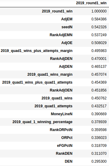
For the first draft of the model, we are going to try to keep things simple and just pick adjEM and Quad1 Wins + Attempts margin. This way we avoid sampling bias by not over-indexing the model by stacking variables that all show a modest correlation when independently measured. Example: we shouldn’t pick adjusted efficiency, defensive efficiency, offensive efficiency, and efficiency ranks because these all make up the adjEM (well, rank is derived from the adjEM so it’s also not a great choice). If a team has an advantage in efficiency margin and Quad1 Wins + Attempts Margin then we are going to place the bet. To keep things simple, let’s assume everything is a $50 bet.
Build the model
Let’s write our model in Python. First we split each game into a couplet – so our DataFrame now has one row with two teams on each line. Then, we convert our data to integers for easier comparison and then we compare the head-to-head adjusted efficiency rates for each team as well as the quad1 wins + attempts on a head-to-head basis. If a team has a better adjusted efficiency margin and more quad 1 wins and attempts, we place the bet! Surely, this will make us millions. We’ve done it. We beat Vegas! Not so fast…
import pandas as pd
import numpy as np
df = pd.read_excel("couplets2.xlsx","Sheet1")
#after import convert float to integers for easier comparison
df["AdjEM"] = pd.to_numeric(df["AdjEM"])
#compare the head to head adjusted efficiencies
df['team1_efficiency_is_better'] = np.where((df['AdjEM'] >= df['adjem2']), 1, 0)
df['team1_more_wins'] = np.where(df['wins'] > df['wins2'], 1, 0)
#compare the head to head quad1 wins + attempts
df['team2_efficiency_is_better'] = np.where((df['AdjEM'] <= df['adjem2']), 1, 0)
df['team2_more_wins'] = np.where(df['wins'] < df['wins2'], 1, 0)
#identify which bets to place
df['make_the_bet_on_team1'] = np.where((df['team1_efficiency_is_better'] + df['team1_more_wins'] >= 2), 1, 0)
df['make_the_bet_on_team2'] = np.where((df['team2_efficiency_is_better'] + df['team2_more_wins'] >= 2), 1, 0)
print(df)
Code language: Python (python)Test the model
Let’s run the model blindly against the actual results of the 2019 tournament and see the results we get. 18 bets placed ($900). Overall record: 12-6. Hey, that’s not too shabby! Unfortunately due to the way the 2019 tournament was seeded, we ended up placing no bets on any underdogs according to the Money Line. Overall, we made -$213.45 or -23.7% return on investment. Yikes! If only it was as easy as correlating the variables, writing a model and then, beating the Vegas odds. Remember, the House always wins. I can just see myself now justifying, saying, “well I just came to Vegas to have fun with friends, so losing $200 is not that bad.”
Baseline our results
Let’s take a step back and build a baseline model to compare our results against. We can see that seed has the second strongest correlation of our set of variables. Let’s compare how we would have done if we just went straight chalk and picked the teams with the lower seeds. Straight chalk, homie!
26 bets placed ($1300). Overall record: 14-12. We placed no bets on any upsets according to the Money Line. Overall, we made -$469.59 or -36.12%. Ouch! So at least my first model is better than just picking the team with the lower seed! I’ll take 13% better return on investment than just picking the lower seed – at least for a first crack!
After doing some data snooping, what if we trim the median, using a 75% interval and try to go totally “anti-chalk” by betting every underdog three seed and above? 22 bets placed ($1100). Overall record 12-10. All 22 bets were placed on underdogs and we won 10 of them. Overall, we made $400.40 or +36%. Great result, but not so fast! This approach is really not based on our model at all and is likely representative of a variety of sampling biases like the vast search effect as well as target shuffling. Basically, by repeatedly running models, cherry-picking data, and changing the target outcome, we find what appears to be a solid approach only for it to fail, catastrophically, when run under real conditions.
If you torture the data long enough, eventually it will confess.
What a bunch of statisticians supposedly say at happy hour.
Said more simply, the fact that the 2019 tournament had 10 upsets in the first round absolutely must be drawn out to a bigger data set to see if this result happens every year (it does not). Just checked the data and going back to 1985, when you trim the median like I did you see somewhere around 6, maybe 7 upsets on average in the first round per year. Unfortunately for my hypothesis, many of these upsets took place by the team with the lower adjusted efficiency and a lower quad 1 wins + attempts margin. As the saying goes, that’s why they play the game and why I suck at data science so far.
Wrapping it all up
So was my model effective? That depends. Do you like to make money when you gamble? Kidding aside, I think a model that was 13% more effective than baseline is a great starting point. But, yes it did lose money. Overall, I’m pleased with my effort, learning, and setting a foundation to improve on next year.
Improving next year
For improving on this model next year we should look to expand the amount of data in the model by looking at games from more than one tournament year. Additionally, we should look to improve the value of the adjusted efficiency and the quad1 wins + attempts variables by more heavily weighting the performance of the teams within the last month or two leading up to the tournament. The way college teams play in the beginning of the year is rarely indicative of how they play at the end of the year. Another good area to focus would be splicing the quad1 data even further. As an example, we can split the quads into eighths by breaking each quad into a “good” game (top half of the quadrant) and a “bad” game (bottom half of the quadrant).
Overall, this was a good and fun first learning project–even though the tournament was canceled. So much learning is in front of me.